Dr.
Gerald S. Hecht
Associate
Professor of Psychology
College
of Sciences
webmaster@psiwebsubr.org
PSYC 4035 - Drugs and Behavior
Exam 2 Study Guide
CHAPTER 2: Research
Design
- Independent
variable: drug
- Dependent
variable: behavior
- Between-subject
designs: different subjects are the source of experimental
control
- uses many subjects
- expensive
- fast
- group averages
- dependent variable only measured once
- Within-subject
designs: same subject's stable baseline behavior measures
are the source of experimental control
- uses fewer subjects
- slower
- dependent variable must be stable
- data from individuals
- no variation due to genetic and individual differences
- Statistical
tests:
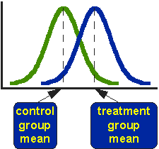
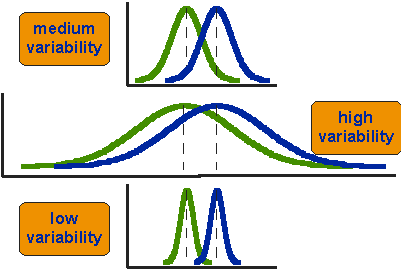
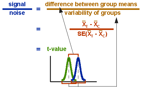
Legitimate drug effects on behavioral measures (signals) must be
separable from chance variations (noise) on behavioral measures over
time (within-subject designs) and from subject to subject
(between-subject designs). These decisions are based on the
probabilities of observing behavioral changes of a given magnitude if
the Independent Variable (drug) was actually doing nothing. Typically
this is achieved using parametric statistics which take advantage of
the fact that normal (gaussian) distributions map onto binomial
probability distributions the limits of the distribution size
approaches infinity.
- Statistical Testing
Basics:

-
The
formula for the normal distribution where:
f (X) = the relative
frequency of a particular score
X = An observed score
µ = the population mean
ð2 = the
population variance
n = the constant pi (3.1416)
e = the base of the natural logarithm
(2.7183)
-
The Normal Distribution approximates the binomial
probability distribution as N (the number of observations)
approaches infinity. This is VERY important because it leads to a
very interesting phenomenon:
-
The Proportion of area
under a given range of the curve equals the probability of randomly
selecting
points in cartesian space in that fall within that area.Remember
Cartesian or
vector algebra is the mapping of points in two dimensions (an X-axis
and
a Y-axis) and then fitting a linear function that best fits those
points.Note the constant pi and think of its use in calculating the
area of a circle (pi multiplied times
the square of the radius)... if you visualize yourself as traveling
"through"
or "around" the curve ("hump") of the normal distribution think about
what
you would see as you "surf the curve"... looking down at the area below
you...the
point is that as two dimensional (X and Y) coordinates are integrated
into
the function one is able to simultaneously calculate
-
PROPORTIONS of
areas covered by regions of distribution AND
-
PROBABILITY
of random observations falling within that area.Now, the hypothetical
Normal Distribution has 4 points of equilibrium (balance points between
opposing forces) about the mean that can be described. Recall from
Calculus that these are known as MOMENTS.Using the moments one
can interpret the meaning of any single score in the distribution in
terms
of probability theory.
- ARITHMETIC MEAN:

- FIRST MOMENT ABOUT THE MEAN:
The sum of the deviation scores divided by the total number of scores (observations)

Not very useful as a measure of dispersion because it is always equal
to 0. Half of the scores will be below the mean (negative numbers) and
the other half will be above the mean (positive numbers) so when you
sum them they cancel each other out and equal 0. Remember a moment is a
point of equilibrium between opposing forces—the mean itself is the
measure of measure of central tendency in a normally distributed
continuous data set—the first moment is 0 units of distance away from
it—the mean itself is the point of equilibrium.
- SUM OF THE SQUARED DEVIATION SCORES (Sum of Squares or SS):

In order to get a useful measure of dispersion around the mean one can
square the deviation scores prior to summing them. This will eliminate
the negative signs from the scores that are below the mean thus
yielding a quantity other than 0.
Importantly, scores that are farther away from the mean have a greater
effect on the sum of squares than scores that are closer to the mean
(e.g. a deviation score of 1 unit squared still equals 1 but a
deviation score of 9 units squared equals 81. Therefore distributions
that are very spread out will have much larger sums of squares than
distributions that are less dispersed. Scores that are the farthest
away from the mean will effect the sum of squares the most. At first,
this seems like a useful measure of dispersion of a distribution—if all
the scores cluster closely about the mean the sum of squares will be
small. If the scores are widely distributed about the mean the sum of
squares will be larger. It is tempting to use this as a measure of
dispersion – small SS’s mean the distribution is less spread out and
large SS’s mean it is very spread out. Unfortunately, however, the SS
is also influenced by the number of scores in the distribution—the more
of them there are the larger the SS will become. This is a source of
contamination that precludes the use of SS as a pure measure of
dispersion.
- THE SECOND MOMENT ABOUT THE MEAN:
The second moment about the mean is also know as variance and is symbolized as

Although, we cannot use the SS as an uncontaminated measure of the
dispersion of scores about the mean, we can divide the SS by the total
number of scores and thereby calculate an average of the squared
deviations. The important point here is that the variance averages the
effects of large and small deviations from the mean and is therefore
not affected by the number of observations in the data set. It is in
fact restricted to your particular data set in the same way that the
arithmetic mean as a measure of central tendency is. Therefore we can
use the variance to characterize how much a randomly selected, typical
score deviates from the mean… it is the first useful measure of
dispersion in a normal distribution… it is our second moment.
Although the variance is a useful
measure of dispersion, it is no longer based on the same units of
measurement as our measure of central tendency (the arithmetic mean)
because all of the deviation scores were squared before dividing them
by the total number of scores. The variance is not interpretable in
terms of our measurement scale. In order to correct the distortion in
measurement resulting from squaring the deviation scores we can now
calculate the square root of the variance. This measure of dispersion
is known as the standard deviation

- WHAT THE FORMULAE FOR THE NORMAL DISTRIBUTION, MEAN AND STANDARD DEVIATION TELL US:
Armed with our formula, our measure of
central tendency and first two moments about the mean we are able to
calculate proportions of area under the normal distribution and thereby
determine the probability (percentile ranking) of any given score on a
measure of behavior (the dependent variable in Drugs and Behavior). In
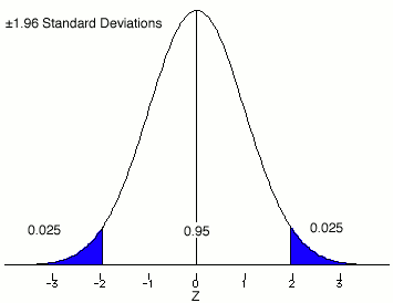
fact the proportion /probability of the area between the mean and + 1
standard deviation = .68 or 68 percent—- between + 2 standard
deviations = .95 or 95 percent—and between + 3 standard deviations =
.997 or 99.7 percent.
- THE THIRD MOMENT ABOUT THE MEAN: SKEW

Skew refers to the symmetry of the distribution. A positive skew means
that the arithmetic mean is larger than the median (from elementary
stats chap 3) and a negative skew means that the arithmetic mean is
smaller than the median. When calculating the magnitude of the third
moment about the mean positive values = a positive skew and negative
values = a negative skew. If the skew = 0 then the distribution is
symmetrical and the mean = the median. Data sets with indices of skew
that range between + 0.50 are considered to be within the limits of
symmetry for calculations of area and percentile ranking with normal
distributions.
- THE FOURTH MOMENT ABOUT THE MEAN: KURTOSIS

The kurtosis is a descriptive measure that tells us whether the scores
are bunched closely around the mean or spread out over a wide range
with many scores in the “tails” of the distribution. Distributions that
are spread out are described as being platykurtic, while those that
cluster tightly about the mean are described as leptokurtic. The
“perfect” normal distribution or classic “bell-shaped” curve is in
between the platy and lepto kurtic extremes—it is known as mesokurtic
and it occurs when

= 3.
We have now reached the point where we
can combine what we know about normal distributions to test various
hypotheses regarding the behavioral effects (Dependent Variable) of
Psychoactive Drugs (Independent Variable) in target populations. We will
do this my calculating the effects of independent variables on
dependent variables in samples and then use the principles of
probability to make inferences about the populations from which our
samples were drawn.
HYPOTHESIS: A statement concerning the
relationship between independent and dependent variables. We will use
several techniques from the field of formal logic to construct our
hypothetical (i.e., concerning the hypothesis) arguments.
- NHST AND THE MODUS TOLLENS PROCEDURE:
The methods of science used in
hypothesis testing never prove anything (despite the cartoon version of
science we get exposed to in movies, TV, etc.). Science uses the formal
logical procedure of modus tollens to evaluate hypotheses. This is a
procedure of falsification based on the fact that a single observation
can lead to the conclusion that the premise or prior statement is
incorrect. In psychological research the modus tollens is constructed
through Null Hypothesis Significance Testing (NHST). In NHST two
statistical hypotheses are created; the null hypothesis (H0) and the alternative hypothesis (H1).
The null hypothesis is presented as the prior statement that is the
“target” of our “falsification attack”. Logically, it is similar to the
American criminal justice model—in which the condition of innocence is
the a priori or null. Only if evidence accumulates during the trial
that is inconsistent with that hypothesis being true, is the null
rejected. In science, our null hypothesis takes the form of the
argument that our Independent Variable (IV) has no effect on our
Dependent Variable (DV). The null hypothesis specifies that the values
of one or more population parameters (DV) do not differ as a function
of exposure to an IV. The alternative hypothesis specifies that the
population parameter under study (DV) is some value other than the one
specified under the null hypothesis. If, at the end of our experiment,
the probability of our DV values (scores—hint, hint) is extremely low
if the null is really true, we reject the null hypothesis as false and
tentatively accept the alternative hypothesis as being a more accurate
reflection of reality.
- EXAMPLE: If H0 is true, then result X would probably not occur.
Result X has occurred.
H0 is probably not true.
H
0 :

H
1:

The null hypothesis states there is no
difference between the two means. If the null hypothesis is false the
researcher should find that difference between the estimated population
means is too large to be accounted for by chance (random) level
probability alone. Therefore, the behavioral pharmacologist has reason
to say the evidence does not support the null hypothesis and it should
be rejected in favor of the alternative hypothesis being tentatively
accepted as a more accurate description of the population parameters.
- REJECTING THE NULL HYPOTHESIS (Details, Details...):
NHST decisions are based on
probabilistic rather than definitive information. The first step
therefore, is to determine a probability level where we are willing to
reject the null hypothesis and tentatively accept the alternative
hypothesis as being more consistent with the data. This point is known
as the alpha level and the cutoff point as the significance level.
ALPHA (

) LEVEL: The level of significance used by the experimenter to decide
if the probability of obtaining certain results on a DV are so unlikely
to occur by chance alone that they warrant rejecting the null
hypothesis.
SIGNIFICANCE LEVEL: The probability
value used to conclude that the null hypothesis is an incorrect
statement. By convention, .05, .01 and .001 are frequently used
significance levels in Psychological research. Failure to reject the
null hypothesis does not mean that the null hypothesis is correct, it
only means that we have not collected sufficient information to reject
it as a false statement. We also have not proved that the alternative
hypothesis is true. When we reject the null hypothesis, we are saying
that the alternative hypothesis provides a more probable explanation
for the data.
PROBABILITY (p) AND ALPHA (

): If: p is less than or equal to alpha then: reject the null
hypothesis in favor of the alternative hypothesis. If: p is greater
than alpha then: fail to reject the null.
- GUESS WHAT? SOMETIMES YOU BET ON THE WRONG HORSE:
Sometimes you reject the null
hypothesis and it was really true. You messed up (Remember those
results could happen by chance 5 times out of 100 if your alpha was set
at p=.05). At least you can know the name given to your mistake—a type
I error (also known as an alpha error).
Other times you fail to reject the null hypothesis but the null
hypothesis really is false—you messed up again—this time you have made
a type II error (also known as a beta error).
- THE SEVEN STEPS FOR HYPOTHESIS TESTING USING THE t-TEST EXAMPLE IN THE BOOK:
STEP 1: State the null hypothesis. H
0:

STEP 2: State the alternative hypothesis. H
1:

STEP 3: Identify the appropriate statistical test. Student’s t-ratio for independent groups.
STEP 4: Determine the significance level. By convention

STEP 5: Identify the appropriate
sampling distribution. Remember all of this is used to make inferences
about the populations from which the samples were drawn.
STEP 6: Identify the critical region for rejection of H0.
These values will come from what you know about probability and the
normal curve, sampling distributions and your significance level.
STEP 7: Summarize and Analyze the data.
- THE ACTUAL FORMULAE FOR THE t-TEST -- SHOWING YOU THE POOLED VARIANCE FILTER AS WELL:
Pooled Variance Formula:

t-Test Denominator Formula:

t-Test Formula itself:

1. The Basic Scenario:

2. The reason for pooled variance considerations:

3. What you have actually determined:

Note that in the "real world" it would
never be this simple -- remember our old friend known as the DRC (dose
response curve) from the last unit. It would never be the case in a
behavioral pharmacology experiment that a single dose of a drug would
be compared with a placebo--you would have a range of doses tested to
generate the DRC. Since the actual alpha level would double with each
successive t-test (separately comparing each dose with the placebo
control), your results would be contaminated by family wise alpha level
inflation. You would need to use more sophisticated statistical
techniques such as ANCOVA (using the placebo condition measures as
covariates, etc.).
- PLACEBO AND RELATED CONCEPTS OF CONTROLS IN BEHAVIORAL PHARMACOLOGY:
Placebo: inert substance given as though it were a drug
Placebo Effects:
- in humans drugs often do what people expect. Behavioral Pharmacology experiments must have a placebo control
- EXPERIMENTER BIAS CONTROLS:
Double-Blind Design - neither the participant nor the experimenter can
know who
is getting the drug and who is getting the placebo.
- THE THREE GROUPS DESIGN FOR TESTING NEW THERAPEUTIC DRUGS:
1. New drug
2. Placebo
3. Established treatment
1X2 = tests hypothesis that New drug has significant effects.
2X3 = tests sensitivity of measurement methods to be used in null hypothesis tests.
1X3 = tests for advantages (i.e., potency, efficacy, TI, side-effect profile) over established treatment.
-
NON-EXPERIMENTAL RESEARCH:
- includes case study method and correlational methods
- at best: can demonstrate correlation, not causality.
- INTROSPECTION AS METHOD FOR MEASURING DEPENDENT VARIABLES:
- unstructured introspection
- "bad" (low reliability & validity). Example: "yo dude...I don't
think this bud is as killer as that last bag...definitely way more
headachy"
- structured introspection -
"good" (can be very high in both reliability and validity). Example:
Methods used in Psychophysics ("eye exam" introspection).
- two examples of "paper and pencil" instruments that are 1) examples
of high quality structured introspection and 2) are highly sensitive to
the effects of psychoactive drugs
1. POMS - Profile of Mood States
2. ARCI - Addiction Research Center Inventory
- BASIC NEUROLOGICAL DEPENDENT VARIABLES USED IN HUMAN BEHAVIORAL PHARMACOLOGY:
- Level of Neural Arousal
- typically a "crude" electrophysiological measure of neural activity (EEG) used to explore:
1. Sleep - stages
2. arousal and mood
3. arousal and activity

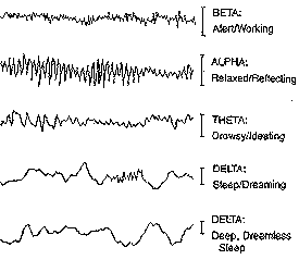
EEG reveals four categories of these brainwaves, ranging from the most activity
to the least activity. When the brain is aroused and actively engaged
in mental activities, it generates beta waves. These beta waves are of
relatively low amplitude, and are the fastest of the four different
brainwaves. The frequency of beta waves ranges from 15 to 40 cycles a
second. Beta waves are characteristics of a strongly engaged mind. A
person in active conversation would be in beta. A debater would be in
high beta. A person making a speech, or a teacher, or a talk show host
would all be in beta when they are engaged in their work.
The
next brainwave category in order of frequency is alpha. Where beta
represented arousal, alpha represents non-arousal. Alpha brainwaves are
slower, and higher in amplitude. Their frequency ranges from 9 to 14
cycles per second. A person who has completed a task and sits down to
rest is often in an alpha state. A person who takes time out to reflect
or meditate is usually in an alpha state. A person who takes a break
from a conference and walks in the garden is often in an alpha state.
The
next state, theta brainwaves, are typically of even greater amplitude
and slower frequency. This frequency range is normally between 5 and 8
cycles a second. A person who has taken time off from a task and begins
to daydream is often in a theta brainwave state. A person who is
driving on a freeway, and discovers that they can't recall the last
five miles, is often in a theta state--induced by the process of
freeway driving. The repetitious nature of that form of driving
compared to a country road would differentiate a theta state and a beta
state in order to perform the driving task safely.
The
final brainwave state is delta. Here the brainwaves are of the greatest
amplitude and slowest frequency. They typically center around a range
of 1.5 to 4 cycles per second. They never go down to zero because that
would mean that you were brain dead. But, deep dreamless sleep would
take you down to the lowest frequency. Typically, 2 to 3 cycles a
second.
It
is a well known fact that humans dream in 90 minute cycles. When the
delta brainwave frequencies increase into the frequency of theta/beta hybrid
brainwaves, active dreaming takes place and often becomes more
experiential to the person. Typically, when this occurs there is rapid
eye movement, which is characteristic of active dreaming. This is
called REM, and is a well known phenomenon.
These patterns of EEG activity used as dependent measures of neural arousal are, again very sensitive to the effects of psychoactive drugs (dare I say it again... the Independent Variable).
- PERFORMANCE BASED DEPENDENT VARIABLES IN BEHAVIORAL PHARMACOLOGY:
- Perception (Psychophysical Methods)
1. Method of Adjustment
* The participant adjust the intensity of the
stimulus until they can either just detect or just not detect a stimulus
* Least accurate, but the fastest
* Example – Person turns a knob until they can just sense tone or just not sense a tone
* Example – using the contrast button or knob on your computer
2. Method of Limits
* The participant is given discrete steps in order controlled by the experimenter
* Example – eye test
* Example, have 8 glasses of water, each with 2 cups
of water and different levels of sugar. Glass 1 has no sugar, glass 2
has ¼ teaspoon (t) of sugar, glass 3 has ½ t of sugar,
glass 4 has 1 t of sugar, etc. and glass 8 has 2 t of sugar.
* Present glasses to individual, starting at
different points going from until participant can just taste or not
taste sugar. Y means can taste, N means can’t taste.
Trial 1Trial 2Trial 3Trial 4
Glass 1N
Glass 2NNN
Glass 3NNNN
Glass 4YYNY
Glass 5YYY
Glass 6YY
Glass 7Y
Glass 8Y
* Why go in both directions (ascending and descending)? To prevent and cancel out the following errors
o Error of habituation
– individuals who keep responding the same way, work on principle that
the stimulus is going to be the same as the last stimulus
+ want to be absolutely sure tasted sugar before responding yes
o Error of anticipation
– individuals who jump the gun and change their responses quickly, work
on principle that the stimulus is going to be different from the last
stimulus
+ as soon as possibility that might has tasted sugar, say yes
3. Method of Constant Stimuli
* The stimuli are randomly presented a number of times
* Slowest, but most accurate
* Example, instead of giving above glasses of water in order, present them to the participant randomly.
* Hearing test
Weber’s Law (just noticeable difference)
• Relates size of JND to size of the standard.
• Difference threshold gets larger as standard gets larger but ratio remains the same
• 
– Delta R = change in physical magnitude needed for difference detection
– R = magnitude of standard stimulus
– k = Weber fraction
• Smaller the fraction, better can discriminate
Common Weber Fractions
• Light intensity 0.079, Sound Intensity 0.048, Lifted Weight 0.022, Line Length 0.029, Taste 0.083, Electric Shock 0.013
Fechner’s formula
• Assume all JND are psychologically equal (60-61 change is same as 300-305 change)
* The relationship fits a logarithmic function for all of the senses S = k log R
* where S=change in sensation (JND),
* R is the magnitude of the physical stimulus
* k is the constant derived from Weber’s law : 
– Perception, constant, intensity
– Log – the power to which 10 must be raised to equal that number (log 10 = 1, log 100 = 2)
- Attention
1. Critical Flicker Fusion (CFF)

The CFF task asseses the integrative capacity of the central nervous
system (CNS), and more specifically, the ability to discriminate
discrete 'bits' of sensory information.
Subjects are required to discriminate flicker from fusion, and vice
versa, in a set of four light emitting diodes arranged in a one
centimetre square. The diodes are held in foveal fixation at a distance
of one metre. Individual thresholds are determined by the
psychophysical method of limits on four ascending (flicker to fusion)
and four descending (fusion to flicker) scales . The mean of these four ascending and descending
presentations gives the threshold frequency in hertz. CFF has been
shown to be sensitive to a variety of psychoactive compounds. A decrease in the CFF threshold is indicative of a reduction in
the overall integrative activity of the CNS.
2. Choice Reaction Time (CRT)

The CRT task is used as an
indicator of sensorimotor performance, assessing the ability to attend
and respond to a critical stimulus . Subjects place the index
finger of their preferred hand on a central starting button, and are
instructed to extinguish one of six equidistant red lights, illuminated
at random, by pressing the response button immediately in front of the
light as quickly as possible. The mean of fifty consecutive
presentations is recorded in milliseconds as a response measure of
three components of reaction time: recognition, motor and total
reaction time. Recognition reaction time (RRT) is the time it takes for
the subject to notice the light, being the time between stimulus onset
and the subject lifting their finger from the start button. Motor
reaction time (MRT) indexes the movement component of this task, and is
the time between the subject lifting their finger from the start button
and touching the response button. The total reaction time (TRT) is the
sum of RRT and MRT. CRT is sensitive to a variety of psychoactive
agents.
- Vigilance
1. Continuous Tracking Test (CTT)

This interactive task of psychomotor function entails using a joystick
control to keep a cursor in alignment with a moving target on a VDU
screen. The movement of the target is a function of of an irregular
sine wave. The response measure (RMS) is the mean difference between
the centres of target and cursor in pixels, sampled 10 times per
second, over the15 minute test. Lower scores are indicative of more
accurate tracking. A peripheral awareness task (PRT) is included in
which the subject responds to a stimulus presented in the periphery of
vision, while simultaneously attending to the tracking test. The mean
reaction time in milliseconds to these stimuli over the trial period is
taken as the response measure for this component of the divided
attention task.
- Motor Performance
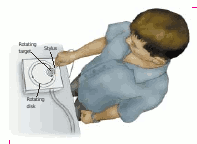
1. Pursuit Rotor
Pursuit-Rotor Task The subject must keep the stylus in contact with
the metal disc that is moving in a circular pattern on a turntable,
which also is moving in a circular pattern. Although the task is
difficult, most people show significant improvement after a brief
period of training. Both initial performance and learning curves with repeated training
sensitive to various psychoactive drugs.2. Hand Steadiness
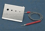
 The
subject’s task is to hold a metal-tipped stylus in 9 progressively smaller
hole sizes without touching the sides. The effects on steadiness of right
vs. left hands, resulting from administration of psychoactive drugs can be
observed and accurately measured.
The
subject’s task is to hold a metal-tipped stylus in 9 progressively smaller
hole sizes without touching the sides. The effects on steadiness of right
vs. left hands, resulting from administration of psychoactive drugs can be
observed and accurately measured.- Driving
1. Real Traffic
'nuff said.
2. Driving Simulator Tests Example: Brake Reaction Time (BRT)
BRT is used as a measure of
cognitive and psychomotor performance including attentional efficiency.
It is assessed in an automatic, dual control car, on a closed circuit.
A red lamp mounted on the bonnet simulates the brake light of an
imaginary vehicle in front of the test car. The lamp is illuminated at
random intervals throughout the test. The subject is required to
extinguish the lamp as quickly as possible, by depressing the brake
pedal. The interval between the illumination of the red light and the
initiation of braking is measured in milliseconds. A microcomputer is
used to control the presentation of the stimuli and to record the
results. Each test consists of 25 BRT trials. The mean latency of BRT
following the illumination of red lamp is recorded. BRT is sensitive to
pychotropic drug effects and provides results, which are consistent
with laboratory measures of reaction times (CRT) and psychomotor
performance.
- MEASURING PERFORMANCE IN NON-HUMAN ANIMAL SUBJECTS:
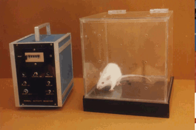
1. SMA - Spontaneous Motor Activity.

The Animal Activity Monitor
incorporates highly sensitive electronic capacitive sensors to detect
changes in vibratory movements on the platform of the animal cage as a
function of psychoactive drug ingestion/administration. The animal is
placed inside an acrylic transparent cage that rests on the sensor
platform. Testing can be conducted in complete darkness,or in bright
sunlight. Ambient illumination is not a limiting factor as in most
photocell activity monitors.It detects ambulatory movements as well as
stereotypic activity like grooming, scratching, digging, etc.
Vibrations caused by the animal activity produce proportional
electrical signals. These are electronically processed to generate
trigger pulses and drive a Digital Counter. Every count registered is
accompanied by a flashing LED and beeper. The sensitivity of the animal
activity monitor is adjustable as per user’s experimental requirements.
An optional Timer is available to programme experiment times from
1 to 99 minutes.
- Respondent Conditioning
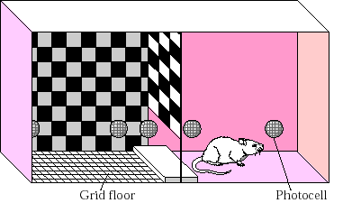
1. Pavlovian conditioning example: Conditioned Place Preference (CPP)
The
apparatus consists of two compartments that vary along several sensory
dimensions,
including the characteristics of the floor and the pattern or color of
the walls. After each compartment has been repeatedly paired with drug
or saline administration,
the reinforcing or aversive effect of the drug is determined in a test
session in which
the animal has access to both compartments, and the amount of time
spent in each is
monitored with photocells or by visual observation.
- Operant Conditioning
1. schedules of reinforcement
- Fixed Ratio Schedule (FR): A set number of correct responses must be made to obtain a reinforcer
- Variable Ratio Schedule (VR): Varied number of correct responses must be made to get a reinforcer
- Fixed Interval Schedule (FI): The first correct response made, after a certain amount of time has elapsed, is reinforced
- Variable Interval Schedule (VI): Reinforcement is given for the first correct response made after a varied amount of time
2. Avoidance Operants:
Signal --> Response -->No shock
Signal --> No Response-->Shock
3. Escape Operants (Sidman Avoidance):
Shock-->Response--->no shock
4. Escape-Avoidance Operants:
Signal --> Response -->No shock
Signal --> No
Response->Shock-->Response-->no shock
5. Punishment Operants:
phase 1: Response -->No shock + Reinforcement
phase 2: Response -->Shock + Reinforcement
6. Drug state discrimination:
Stimulus Properties of Drugs
- drugs can act as discriminative stimuli
- can be used to investigate new drugs
- can be used to investigate physiological mechanisms responsible for
the
subjective effect of a drug.
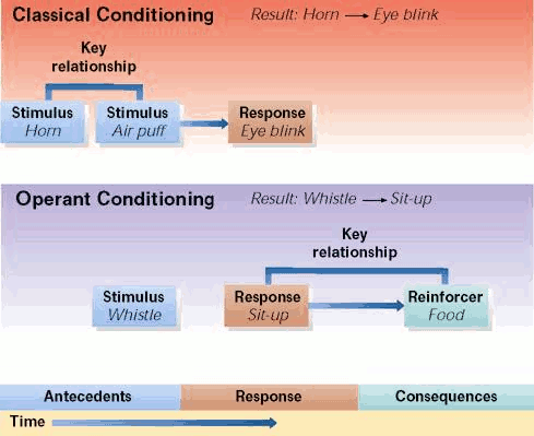
- Summary of Differences Between Respondent (Pavlovian) and Operant Learning:

- Drug Development and Testing:
1. initial screening - nonhuman testing
ED50 and LD50
2. phase 1 - human testing
Toxicity and side effects
3. phase 2 - tested on patients
4. phase 3 - Clinical trials
3 groups design
5. phase 4 - extended data collection
often no compulsory reporting of
side effects.


 = 3.
= 3.


 ) LEVEL: The level of significance used by the experimenter to decide
if the probability of obtaining certain results on a DV are so unlikely
to occur by chance alone that they warrant rejecting the null
hypothesis.
 ): If: p is less than or equal to alpha then: reject the null
hypothesis in favor of the alternative hypothesis. If: p is greater
than alpha then: fail to reject the null.


